PyTorch Layer 이해하기
Load Packages
1
2
3
4
5
6
| import torch
from torchvision import datasets, transforms
import numpy as np
import matplotlib.pyplot as plt
%matplotlib inline
|
예제 불러오기
1
2
3
4
5
6
7
8
9
10
11
| train_loader = torch.utils.data.DataLoader(
datasets.MNIST('dataset', train=True, download=True,
transform=transforms.Compose([
transforms.ToTensor()
])),
batch_size=1)
image, label = next(iter(train_loader))
image.shape, label.shape
=> (torch.Size([1, 1, 28, 28]), torch.Size([1]))
|
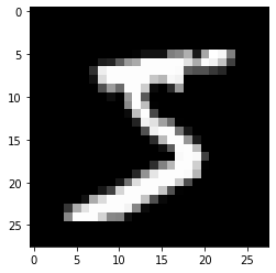
1
2
| plt.imshow(image[0, 0, :, :], 'gray')
plt.show()
|
각 Layer별 설명
Network 쌓기 위한 준비를 합니다.
1
2
3
| import torch
import torch.nn as nn
import torch.nn.functional as F
|
Convolution
- in_channels : 받게 될 channel의 갯수
- out_channels : 보내고 싶은 channel의 갯수
- kernel_size : 만들고 싶은 kernel(weights)의 사이즈
1
2
3
4
|
layer = nn.Conv2d(in_channels=1, out_channels=20, kernel_size=5, stride=1).to(torch.device('cpu'))
=> Conv2d(1, 20, kernel_size=(5, 5), stride=(1, 1))
|
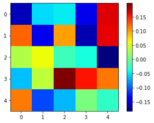
weight 시각화를 위해 slice하고 numpy화 합니다.
1
2
3
4
| weight = layer.weight
weight.shape
=> torch.Size([20, 1, 5, 5])
|
- 여기서 weight는 학습 가능한 상태이기 때문에 바로 numpy로 뽑아낼 수 없다.
- detach() method는 그래프에서 잠깐 꺼내서 gradient에 영향을 받지 않게 한다.
1
2
3
4
| weight = weight.detach().numpy()
weight.shape
=> (20, 1, 5, 5)
|
1
2
3
| plt.imshow(weight[0, 0, :, :], 'jet')
plt.colorbar()
plt.show()
|
- output 시각화 준비를 위해 numpy화 합니다.
1
2
3
4
5
6
| output_data = layer(image)
output_data = output_data.data
output = output_data.cpu().numpy()
output.shape
=> (1, 20, 24, 24)
|
- input으로 들어간 이미지 numpy화 한다.
1
2
3
4
| image_arr = image.numpy()
image_arr.shape
=> (1, 1, 28, 28)
|
1
2
3
4
5
6
7
8
9
10
11
| plt.figure(figsize=(15, 30))
plt.subplot(131)
plt.title('Input')
plt.imshow(np.squeeze(image_arr), 'gray')
plt.subplot(132)
plt.title('Weight')
plt.imshow(weight[0, 0, :, :], 'jet')
plt.subplot(133)
plt.title('Output')
plt.imshow(output[0, 0, :, :], 'gray')
plt.show()
|
Pooling
input을 먼저 앞에 넣고, 뒤어 kernel 사이즈와 stride를 순서대로 넣는다.
1
2
3
4
| pool = F.max_pool2d(image, 2, 2)
pool.shape
=> torch.Size([1, 1, 14, 14])
|
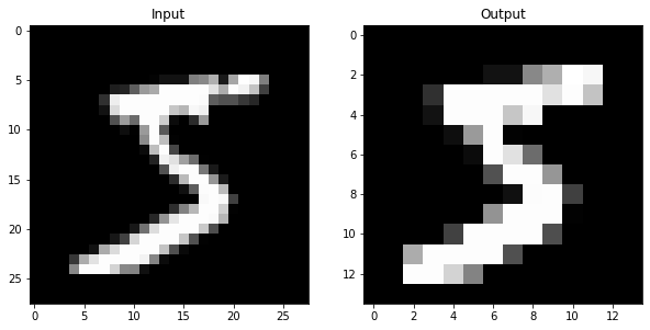
MaxPool Layer는 weight가 없기 때문에 바로 numpy() 사용 가능하다.
1
2
3
4
| pool_arr = pool.numpy()
pool_arr.shape, image_arr.shape
=> ((1, 1, 14, 14), (1, 1, 28, 28))
|
1
2
3
4
5
6
7
8
| plt.figure(figsize=(10, 15))
plt.subplot(121)
plt.title("Input")
plt.imshow(np.squeeze(image_arr), 'gray')
plt.subplot(122)
plt.title('Output')
plt.imshow(np.squeeze(pool_arr), 'gray')
plt.show()
|
Linear
nn.Linear는 2D가 아닌 1D만 들어가기 때문에 view() 함수를 사용하여 1D로 펼쳐줘야 한다.
1
2
3
4
5
|
flatten = image.view(1, 28 * 28)
flatten.shape
=> torch.Size([1, 784])
|
1
2
3
4
5
6
7
8
9
| lin = nn.Linear(784, 10)(flatten)
lin.shape
=> torch.Size([1, 10])
lin
=> tensor([[-0.1198, 0.2404, -0.0522, -0.3474, -0.3997, -0.0318, -0.0630, 0.2680,
0.1849, 0.1000]], grad_fn=<AddmmBackward>)
|
1
2
| plt.imshow(lin.detach().numpy(), 'jet')
plt.show()
|
Softmax
결과를 numpy로 꺼재기 위해선 weight가 담긴 Linear에 weight를 꺼줘야 한다.
1
2
3
4
5
6
7
8
9
| with torch.no_grad():
flatten = image.view(1, 28 * 28)
lin = nn.Linear(784, 10)(flatten)
softmax = F.softmax(lin, dim=1)
softmax
=> tensor([[0.0846, 0.1084, 0.0792, 0.1265, 0.1004, 0.0897, 0.0990, 0.1113, 0.1239,
0.0769]])
|
1
2
| np.sum(softmax.numpy())
=> 0.99999994
|
Layer 쌓기
예제 출처 : https://pytorch.org/tutorials/beginner/pytorch_with_examples.html#id23
nn 과 nn.functional의 차이점
- nn은 학습 파라미터가 담긴 것
- nn.functional은 학습 파라미터가 없는 것
1
2
3
4
5
6
7
8
9
10
11
12
13
14
15
16
17
18
19
20
21
| class Net(nn.Module):
def __init__(self):
super(Net, self).__init__()
self.conv1 = nn.Conv2d(1, 20, 5, 1)
self.conv2 = nn.Conv2d(20, 50, 5, 1)
self.fc1 = nn.Linear(4 * 4 * 50, 500)
self.fc2 = nn.Linear(500, 10)
def forward(self, x):
x = F.relu(self.conv1(x))
x = F.max_pool2d(x, 2, 2)
x = F.relu(self.conv2(x))
x = F.max_pool2d(x, 2, 2)
x = x.view(-1, 4 * 4 * 50)
x = F.relu(self.fc1(x))
x = self.fc2(x)
return F.log_softmax(x, dim=1)
|
image를 Model에 넣어서 결과를 확인한다.
1
2
3
4
5
| model = Net()
result = model.forward(image)
=> tensor([[-2.3262, -2.2901, -2.2722, -2.2262, -2.3148, -2.3693, -2.2773, -2.2977,
-2.3222, -2.3371]], grad_fn=<LogSoftmaxBackward>)
|